선형 AutoEncoder를 활용한 이미지 축소 및 복원
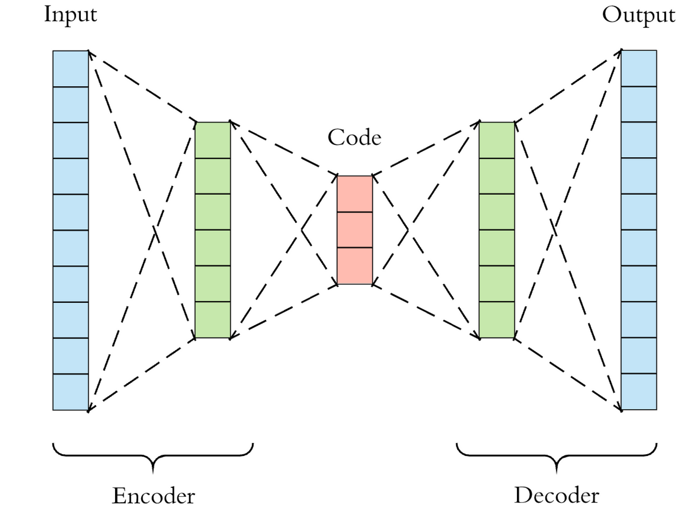
(MNIST 데이터셋 사용)
라이브러리 가져오기
import tensorflow as tf
from tensorflow.keras.models import Sequential, Model
from tensorflow.keras.layers import Dense, Input
import numpy as np
import matplotlib.pyplot as plt
tf.__version__
데이터셋 가져오기
from tensorflow.keras.datasets import mnist

(X_train, y_train), (X_test, y_test) = mnist.load_data()
X_train.shape, y_train.shape #((60000, 28,28), (60000,))
X_test.shape, y_test.shape #((10000, 28,28), (10000,))
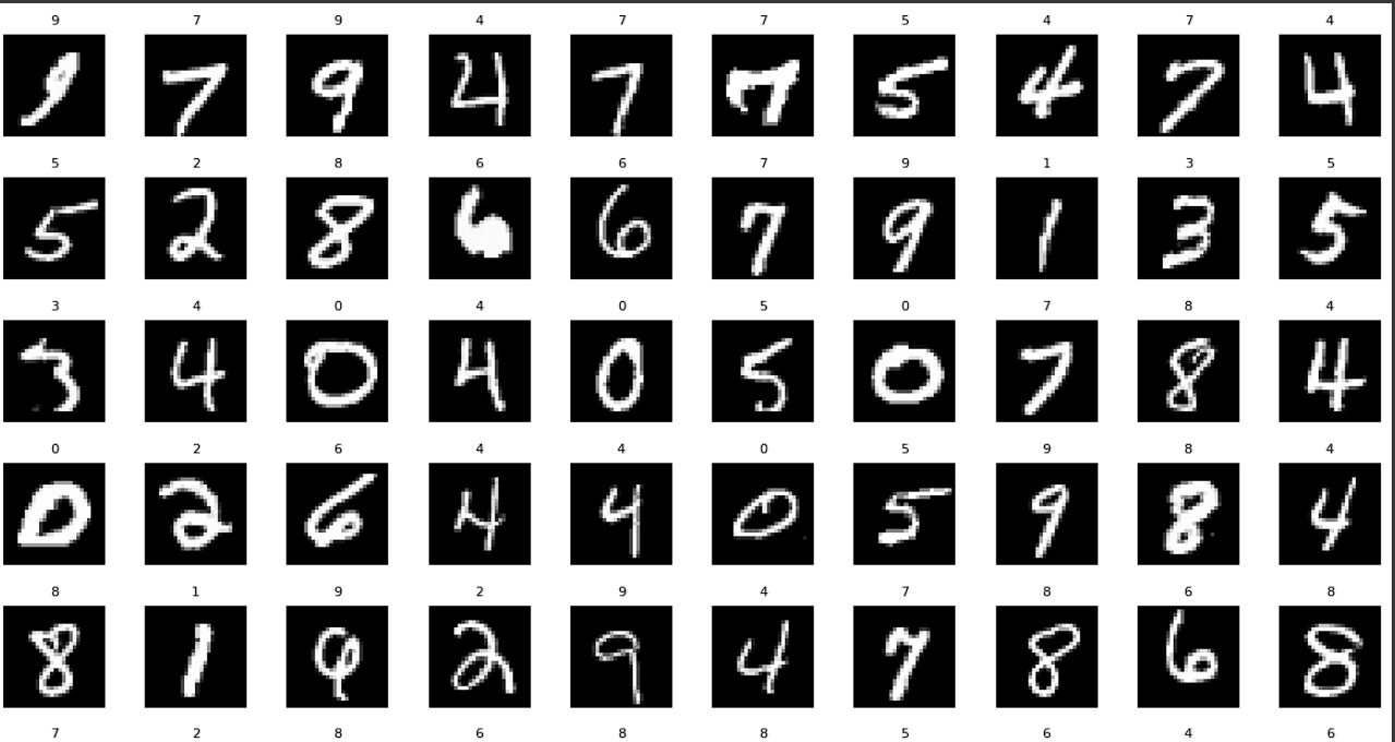
데이터셋 시각화
w, h = 10, 10
f, ax = plt.subplots(h, w, figsize=(15,15))
ax = ax.ravel() # (10, 10) -> (100,)로 벡터화
for i in np.arange(0, w*h):
    index = np.random.randint(0, 59999)
    ax[i].imshow(X_train[index], cmap='gray')
    ax[i].set_title(y_train[index], fontsize=8)
    ax[i].axis('off')
 plt.subplots_adjst(hspace=.4) # horizon space 조정
데이터 전처리
1. 이 데이터셋의 픽셀은 0~255의 숫자로 표현되어 있다. 신경망에 투입하기 전에 꼭 스케일링 작업을 해야한다.
X_train = X_train / 255
X_test = X_test / 255
2. Linear autoencoder를 사용하기 위해선 한 줄의 벡터로 표현을 해줘야 한다.
X_train = X_train.reshape(X_train.shape[0], X_train.shape[1] * X_train.shape[2])
X_train.shape # (60000, 784)

X_test = X_test.reshape(X_test.shape[0], X_test.shape[1] * X_test.shape[2])
X_test.shape # (10000, 784)
모델 훈련
데이터셋과 전처리가 끝났으니 모델을 정의하고 훈련시킨다. Input 784부터, 128, 64, 32 로 축소를 시킨 후, 64, 128, 784로 복원을 한다.
# 일련의 순차 신경망
autoencoder = Sequential()

# encode
autoencoder.add(Dense(units=128, activation='relu', input_dim=784))
autoencoder.add(Dense(units=64, activation='relu'))
autoencoder.add(Dense(units=32, activation='relu'))

# decode
autoencoder.add(Dense(units=64, activation='relu'))
autoencoder.add(Dense(units=128, activation='relu'))
autoencoder.add(Dense(units=784, activation='sigmoid'))
decode 부분에서 마지막 레이어에서 activation='sigmoid'로 했다. 그 이유는 이전에 입력 데이터를 [0,1]로 스케일링을 했고, 이를 복원해야 하기 때문이다.
autoencoder.summary()

'''
Model: "sequential_1"
_________________________________________________________________
 Layer (type)                Output Shape              Param #
=================================================================
 dense (Dense)               (None, 128)               100480

 dense_1 (Dense)             (None, 64)                8256

 dense_2 (Dense)             (None, 32)                2080

 dense_3 (Dense)             (None, 64)                2112

 dense_4 (Dense)             (None, 128)               8320

 dense_5 (Dense)             (None, 784)               101136

=================================================================
Total params: 222384 (868.69 KB)
Trainable params: 222384 (868.69 KB)
Non-trainable params: 0 (0.00 Byte)
_________________________________________________________________
'''
이렇게 6개의 층으로 구성되어 있고, 모델 컴파일 진행한다.
autoencoder.compile(optimizer='adam', loss='binary_crossentropy', metrics=['accuracy'])
모델 훈련
autoencoder.fit(X_train, X_train, epochs=50)
주의 . 입력 데이터를 학습하고 최종적으로 복원하는 과정에서 그대로 입력 데이터가 출력되길 바란다. 그래서 파라미터를 X_train, X_train으로 두었다.
Epoch 1/50
1875/1875 [==============================] - 11s 4ms/step - loss: 0.1567 - accuracy: 0.0113
Epoch 2/50
1875/1875 [==============================] - 7s 4ms/step - loss: 0.1127 - accuracy: 0.0128
Epoch 3/50
1875/1875 [==============================] - 7s 4ms/step - loss: 0.1037 - accuracy: 0.0127
.
.
.
Epoch 49/50
1875/1875 [==============================] - 7s 4ms/step - loss: 0.0821 - accuracy: 0.0138
Epoch 50/50
1875/1875 [==============================] - 8s 4ms/step - loss: 0.0821 - accuracy: 0.0141
<keras.src.callbacks.History at 0x7d2315dd9750>
모델 학습 완료. 여기서, 정확도는 중요하지 않다. 우리가 원하는 건 복원이지 숫자가 어떤 숫자인지 맞추는 classification 문제가 아니다.
이미지 인코딩 & 디코딩
모델이 학습했으니, 테스트 데이터셋을 인코딩 및 디코딩 한다.
from tensorflow.keras.models import Model
autoencoder.input
#<KerasTensor: shape=(None, 784) dtype=float32 (created by layer 'dense_input')>
# encoder
encoder = Model(inputs=autoencoder.input, outputs=autoencoder.get_layer('dense_2').output)autoencoder.summary()에서 봤듯, 'dense_2' 명을 가진 레이어가 인코딩 모델에서는 output이다.
encoder.summary()

'''
Model: "model_1"
_________________________________________________________________
 Layer (type)                Output Shape              Param #
=================================================================
 dense_input (InputLayer)    [(None, 784)]             0

 dense (Dense)               (None, 128)               100480

 dense_1 (Dense)             (None, 64)                8256

 dense_2 (Dense)             (None, 32)                2080

=================================================================
Total params: 110816 (432.88 KB)
Trainable params: 110816 (432.88 KB)
Non-trainable params: 0 (0.00 Byte)
_________________________________________________________________
'''
인코딩 모델을 지정했으니 테스트셋 중 하나를 인코딩해본다.
# 첫 번째 이미지 인코딩(차원 축소)
encoded_image = encoder.predict(X_test[0].reshape(1, -1))
encoded_image, encoded_image.shape

'''
1/1 [==============================] - 0s 76ms/step
(array([[2.5691762, 0.       , 0.       , 0.       , 5.038651 , 4.666224 ,
         0.       , 2.0804176, 2.8104665, 0.       , 2.2300448, 1.3183982,
         1.7357508, 5.5573163, 4.5667076, 5.974587 , 3.205965 , 0.       ,
         5.006193 , 1.7097998, 2.421267 , 5.9979563, 0.       , 5.582242 ,
         6.022785 , 2.8267446, 2.3152354, 9.577605 , 3.4995344, 6.357731 ,
         2.2016535, 6.2968473]], dtype=float32),
 (1, 32))
 '''
reshape(1, -1)로 한 이유가 뭘까? 위 encoder.summary()를 보면 input layer에서 output이 [(None, 784)]인데, 2D shape이다. 기존 (784,)를 (1, 784)로 만든 것이다.
# 인코딩된 이미지 시각화 -> 32 pixel
plt.imshow(encoded_image.reshape(8,4), cmap='gray')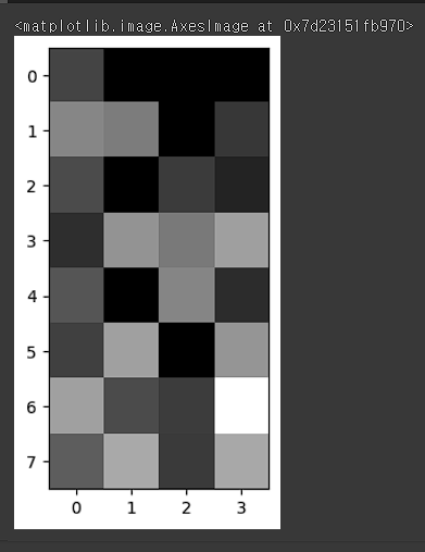
디코딩
이미지를 압축했으니 복원을 하자.
autoencoder.summary()

'''
Model: "sequential_1"
_________________________________________________________________
 Layer (type)                Output Shape              Param #
=================================================================
 dense (Dense)               (None, 128)               100480

 dense_1 (Dense)             (None, 64)                8256

 dense_2 (Dense)             (None, 32)                2080

 dense_3 (Dense)             (None, 64)                2112

 dense_4 (Dense)             (None, 128)               8320

 dense_5 (Dense)             (None, 784)               101136

=================================================================
Total params: 222384 (868.69 KB)
Trainable params: 222384 (868.69 KB)
Non-trainable params: 0 (0.00 Byte)
_________________________________________________________________
'''
# decoder에서 input layer을 정의해야한다.
input_layer_decoder = Input(shape=(32,))
decoder_layer1 = autoencoder.layers[3] # dense_3
decoder_layer2 = autoencoder.layers[4] # dense_4
decoder_layer3 = autoencoder.layers[5] # dense_5
decoder = Model(inputs=input_layer_decoder,
outputs= decoder_layer3(decoder_layer2(decoder_layer1(input_layer_decoder))))
decoder.summary()
'''
Model: "model_2"
_________________________________________________________________
Layer (type) Output Shape Param #
=================================================================
input_2 (InputLayer) [(None, 32)] 0
dense_3 (Dense) (None, 64) 2112
dense_4 (Dense) (None, 128) 8320
dense_5 (Dense) (None, 784) 101136
=================================================================
Total params: 111568 (435.81 KB)
Trainable params: 111568 (435.81 KB)
Non-trainable params: 0 (0.00 Byte)
_________________________________________________________________
'''
decoder_layer를 인덱스로 불러올 수 있으며, decoder 변수의 outputs은 레이들을 연결하기 위한 방법으로 쓰인 것이다.
# 인코딩된 이미지 디코딩
decoded_image = decoder.predict(encoded_image)

# (1,784)
decoded_image.shape
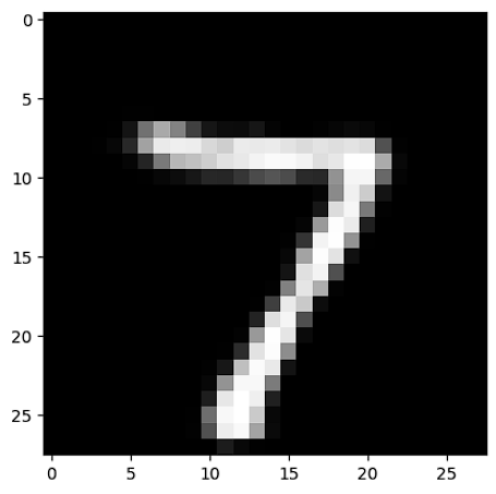
# label
plt.imshow(X_test[0].reshape(28,28), cmap='gray')

# prediction
plt.imshow(decoded_image.reshape(28,28), cmap='gray')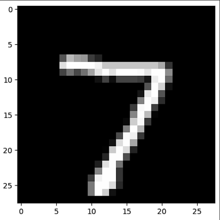
이제, 10장의 이미지를 랜덤으로 가져와서 인코딩 및 디코딩을 거친 후, 비교해보자.
n_images = 10
test_images = np.random.randint(0, X_test.shape[0]- 1, size=n_images)
plt.figure(figsize=(18,18))

for i, image_index in enumerate(test_images):
  # original image
  ax = plt.subplot(10,10, i + 1)
  plt.imshow(X_test[image_index].reshape(28,28), cmap='gray')
  plt.xticks(())
  plt.yticks(())

  # autoencoder
  ax = plt.subplot(10, 10, i + 1 + n_images)
  encoded_image = encoder.predict(X_test[image_index].reshape(1,-1))
  plt.imshow(encoded_image.reshape(8,4),cmap='gray')
  plt.xticks(())
  plt.yticks(())

  # decoded image
  ax = plt.subplot(10, 10, i + 1 + n_images * 2)
  plt.imshow(decoder.predict(encoded_image).reshape(28,28),cmap='gray')
  plt.xticks(())
  plt.yticks(())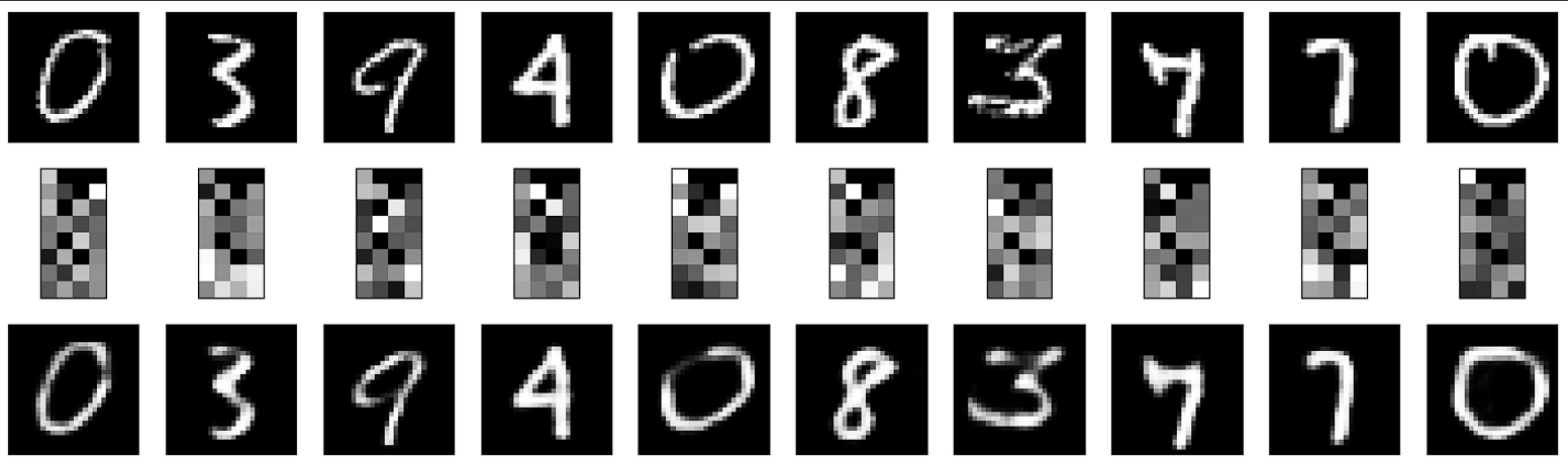
끝.
'DL > Computer Vision' 카테고리의 다른 글
| Computer Vision - [CNN with tensorflow] (0) | 2024.02.20 |
|---|---|
| Computer Vision - [얼굴 인식 2 (Face Recogintion using dlib, shape predictor 68 face landmarks)] (0) | 2024.02.07 |
| Computer Vision - [얼굴 인식 (Face Recogintion)] (1) | 2024.02.01 |
| Computer Vision - [Fruit and Vegetable Classification] (1) | 2024.01.29 |
| Computer Vision - [CNN (Convolutional Neural Network)] (1) | 2024.01.26 |