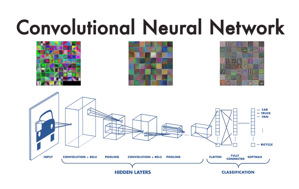
CNN(Convolution Neural Network)를 활용해 호머와 심슨을 분류해보자.
1. Import the library
import matplotlib.pyplot as plt
import seaborn as sns
import zipfile
import numpy as np
from google.colab.patches import cv2_imshow
import tensorflow as tf
from tensorflow.keras.models import Sequential
from tensorflow.keras.layers import Conv2D, Dense, Flatten, MaxPool2D
from tensorflow.keras.preprocessing.image import ImageDataGenerator
tf.__version__ # 2.15.0
2. Load the images
dataset : https://www.kaggle.com/datasets/aasousa/images-simpsons
Images of Simpsons: Homer and Bart
Images of Homer and Bart to classification with Convolutional Neural Network
www.kaggle.com
# google drive
from google.colab import drive
drive.mount('/content/drive')

# homer bart dataset
path = '~/homer_bart_2.zip'
zip_object = zipfile.ZipFile(file=path, mode='r')
zip_object.extractall('./')
zip_object.close()
tf.keras.preprocessing.image.load_img("./bart100.bmp')
3. dataset generator
# 어떻게 데이터셋을 생성할 것인가?
training_generator = ImageDataGenerator(rescale=1./255, rotation_range=7, horizontal_flip=True, zoom_range=2)
test_generator = ImageDataGenerator(rescale=1./255)

# 데이터셋 정의
train_dataset = training_generator.flow_from_directory('/homer_bart_2/training_set',
  target_size=(64,64), batch_size=8, class_mode='categorical', shuffle=True)
test_dataset = test_generator.flow_from_directory('/homer_bart_2/test_set',
target_size=(64,64), batch_size=1, class_mode='categorical', shuffle=False)Found 215 images belonging to 2 classes.
Found 54 images belonging to 2 classes.
- training_generator에는 데이터 증강을 해주지만, test_generator에는 scale만 조정해준다. training dataset을 학습하지
test dataset은 학습할 필요가 없기 때문이다. 이후 데이터를 정의해준다.
- flow_from_directory를 하면 해당 경로 하위 폴더들을 사용한다. bart, homer 폴더가 있기 때문에 binary task가 된다.
- target_size로 사이즈를 동일하게 정의해준다. 해당 폴더 내 이미지들은 size가 달라, batch_size는 8로, 8개의 이미지를 가지고 신경망에 투입한 후, 다음 8장을 가져와 신경망에 또 투입힌다. 이 과정에서 가중치는 업데이트 된다.
- class_mode는 'binary'해도 되지만, 'categorical'로 해도 상관없다. 이진 분류가 아닌 다중 분류라면 'categorical'은 필수다.
- shuffle은 데이터셋을 섞는다. 데이터의 순서가 학습에 영향을 줄 수 있기 때문에 섞어준다.
- train_dataset과 test_dataset은 다르다. batch_size=1로 한 이유는 한 장씩 확인하기 위해서고, shuffle=False는 test data는 학습에 쓰이지 않기 때문에 False로 해준다.
print(train_dataset.class_indices)
print(test_dataset.class_indices){'bart': 0, 'homer': 1}
{'bart': 0, 'homer': 1}
4. Modeling
model = Sequential()

model.add(Conv2D(filters=32, kernel_size=(3,3), strides=(1,1), activation='relu', input_shape=(64,64,3)))
model.add(MaxPool2D(pool_size=(2,2)))

model.add(Conv2D(filters=32, kernel_size=(3,3), strides=(1,1), activation='relu'))
model.add(MaxPool2D(pool_size=(2,2)))

model.add(Conv2D(filters=32, kernel_size=(3,3), strides=(1,1), activation='relu'))
model.add(MaxPool2D(pool_size=(2,2)))

model.add(Flatten()) #행렬 -> 벡터

model.add(Dense(units=577, activation='relu'))
model.add(Dense(units=577, activation='relu'))
model.add(Dense(units=2, activation='softmax'))
model.summary()
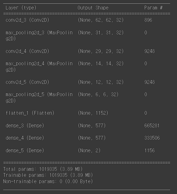
Dense층에서 units 577을 한 이유는 (input의 값 + output 값) / 2 의 값이다. Dense층 앞 input값을 보면 1152이고 output은 2다.
model.compile(optimizer='adam', loss='categorical_crossentropy', metrics=['accuracy'])

# fit_generator 사용
history = model.fit_generator(train_dataset, epochs=50)
Epoch 1/50
27/27 [==============================] - 6s 39ms/step - loss: 0.6662 - accuracy: 0.6140
.
.
.
Epoch 49/50
27/27 [==============================] - 0s 18ms/step - loss: 0.1475 - accuracy: 0.9488
Epoch 50/50
27/27 [==============================] - 0s 18ms/step - loss: 0.0756 - accuracy: 0.9628
accuracy가 0.96으로 나왔다. train dataset 기준으로 구한 것이라 높다. test data로 검증을 해봐야 한다.
5. Evalution
test_dataset.class_indices # {'bart':0, 'homer':1}

predictions = model.predict(test_dataset)
predictions = np.argmax(predictions, axis=1)

cm = confusion_matrix(test_dataset.classes, predictions)
sns.heatmap(cm, annot=True)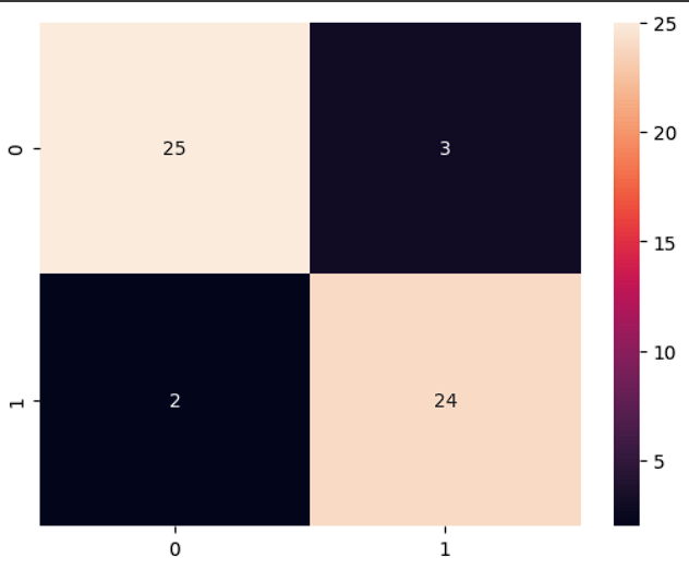
6. Model save & Load
# 1. json 저장으로 신경망 모델 구조를 저장하자.
model_json = model.to_json()
with open('model.json', 'w') as json_file:
  json_file.write(model_json)

# 2. keras로 모델 가중치 저장하자.
from keras.models import save_model
model_saved = save_model(model, './weights.hdf5')

# 3. open json! 다시 모델 구조를 불러오자.
with open('model.json', 'r') as json_file:
  json_saved_model = json_file.read()

# 4. open weights! 다시 모델 가중치를 불러오자.
model_loaded = tf.keras.models.model_from_json(json_saved_model)
model_loaded.load_weights('weights.hdf5')
model_loaded.compile(loss='categorical_crossentropy', optimizer='adam', metrics=['accuracy'])
model_loaded_summary()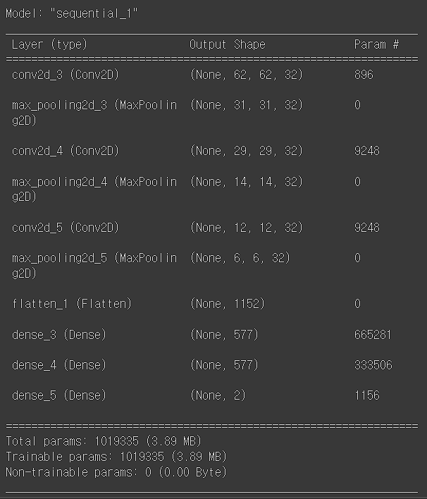
마지막으로 한 장을 예측해보자.
import cv2
image = cv2.imread('homer7.bmp')
cv2_imshow(image)
image = cv2.resize(image, (64,64))
cv2_imshow(image)
image = image/255
print(image.shape)
# (64,64, 3)

image = image.reshape(-1, 64, 64, 3) # 한 장이라 -1로 지정함. 10장을 예측하려면 10으로 두면 됨.
print(image_shape)
# (1, 64, 64, 3)
test_dataset.class_indices
# {'bart': 0, 'homer': 1}

result = model.predict(image)
result = np.argmax(result)
result
1/1 [==============================] - 0s 18ms/step
1
homer로 잘 예측했다.
'DL > Computer Vision' 카테고리의 다른 글
| Computer Vision - [선형 AutoEncoder를 활용한 이미지 축소 및 복원] (1) | 2024.02.27 |
|---|---|
| Computer Vision - [얼굴 인식 2 (Face Recogintion using dlib, shape predictor 68 face landmarks)] (0) | 2024.02.07 |
| Computer Vision - [얼굴 인식 (Face Recogintion)] (1) | 2024.02.01 |
| Computer Vision - [Fruit and Vegetable Classification] (1) | 2024.01.29 |
| Computer Vision - [CNN (Convolutional Neural Network)] (1) | 2024.01.26 |